Benchmarking pandas against Polars from a pandas PoV

Or: How writing efficient pandas code matters

Introduction

I've regularly seen benchmarks that show how much faster Polars is compared to pandas. The fact that Polars is faster than pandas is not too surprising since it is multithreaded while pandas is mostly single-core. The big difference surprises me though. That's why I decided to take a look at the pandas queries that were used for the benchmarks.

I was curious to find out whether there was room for improvement. This post will detail a couple of easy steps that I took to speed up pandas code. The pandas performance improvements are quite impressive!

We will look at the tpch benchmarks from the Polars repository with scale_1 including I/O time.

Fair warning: I had to try this a couple of times since the API changed. You can switch to version 0.17.15, if you encounter problems, that's what I used. Additionally, I am using the current development version of pandas because some optimizations for Copy-on-Write and the Pyarrow dtype_backend were added after 2.0 was released. The development version was also used to create the baseline plots, so all performance gains shown in here can be attributed to the refactoring steps. You can use this version starting from August at the latest!

I came away with one main takeaway:

• Writing efficient pandas code matters a lot.

I have a MacBook Air with M2 processors and 24GB of RAM. The benchmarks are only run once in default mode. I repeated the calculations 15 times and used the mean as result.

Baseline

I ran the benchmarks "as is" as a first step to get the status-quo.

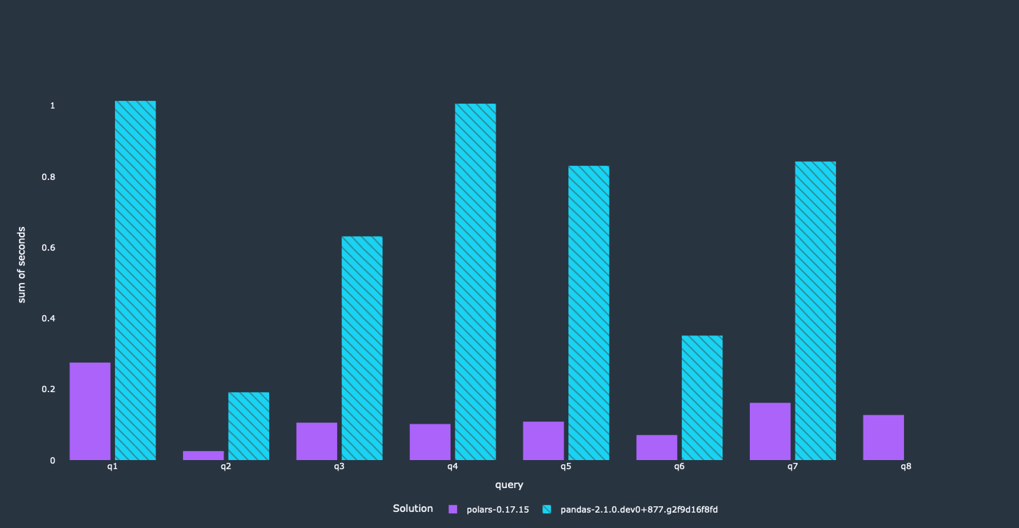
It's relatively easy to see that Polars is between 4–10 times faster than pandas. After getting these results I decided to look at the queries that were used for pandas. A couple of relatively straightforward optimizations will speed up our pandas code a lot. Additionally, we will get other benefits out of it as well, like a significantly reduced memory footprint.

Side note: Number 8 is broken, so no result there.

Initial refactoring

One thing that stood out is that the whole parquet files were read even though most queries only needed a small subset. Some queries also did some operations on the whole dataset and dropped the columns later on. A filtering operation is slowed down quite a bit when performed on the full DataFrame compared to only a fraction of the columns, e.g.:

new_df = df[mask]
new_df = df[["a", "b"]]

This is significantly slower than restricting the DataFrame to the relevant subset beforehand:

df = df[["a", "b"]]
new_df = df[mask]

There is no need to read these columns at all, if they are not used somewhere within your code. Pushing the column selection into read_parquet is easy, since this is offered by PyArrow through the columns keyword.

df = pd.read_parquet(...)
df = df[df.a > 100]
df[["a", "b"]]

This is rewritten into:

df = pd.read_parquet(..., columns=["a", "b"])
df = df[df.a > 100]

I've also turned Copy-on-Write on. It's now in a state that it shouldn't have many performance problems while it will most likely give a speedup. That said, the difference here is not too big, since the benchmarks are GroupBy and merge heavy, which aren't really influenced by CoW. This was a quick refactoring effort that took me around 30 minutes for all queries. Most queries restricted the DataFrame later on anyway, so it was mostly a copy-paste exercise.

Let's look at the results:

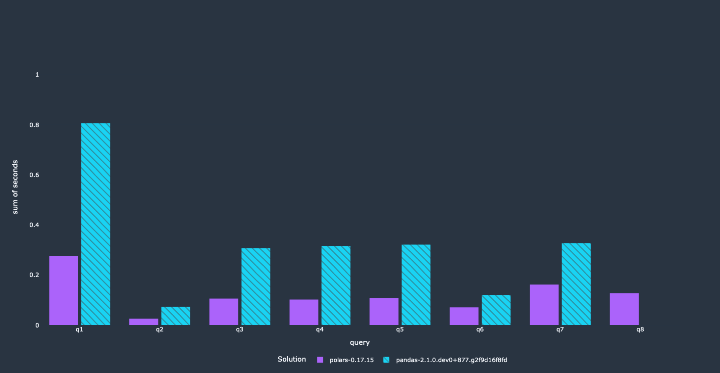
The pandas queries got a lot faster through a couple of small modifications, e.g. we can see performance improvements by a factor of 2 and more. Since this avoids loading unnecessary columns completely, we reduced the memory footprint of our program significantly.

Further optimizations - leveraging Arrow

A quick profiling showed that the filter operations were still a bottleneck for a couple of queries. Fortunately, there is an easy fix. read_parquet passes potential keywords through to PyArrow and Arrow offers the option to filter the table while reading the parquet file. Moving these filters up gives a nice additional improvement.

df = pd.read_parquet(..., columns=["a", "b"])
df = df[df.a > 100]

We can easily pass the filter condition to Arrow to avoid materializing unnecessary rows:

import pyarrow.compute as pc


df = pd.read_parquet(..., columns=["a", "b"], filters=pc.field("a") > 100)

Arrow supports an Expression style for these filter conditions. You can use more or less all filtering operations that would be available in pandas as well. Let's look at what this means performance-wise.

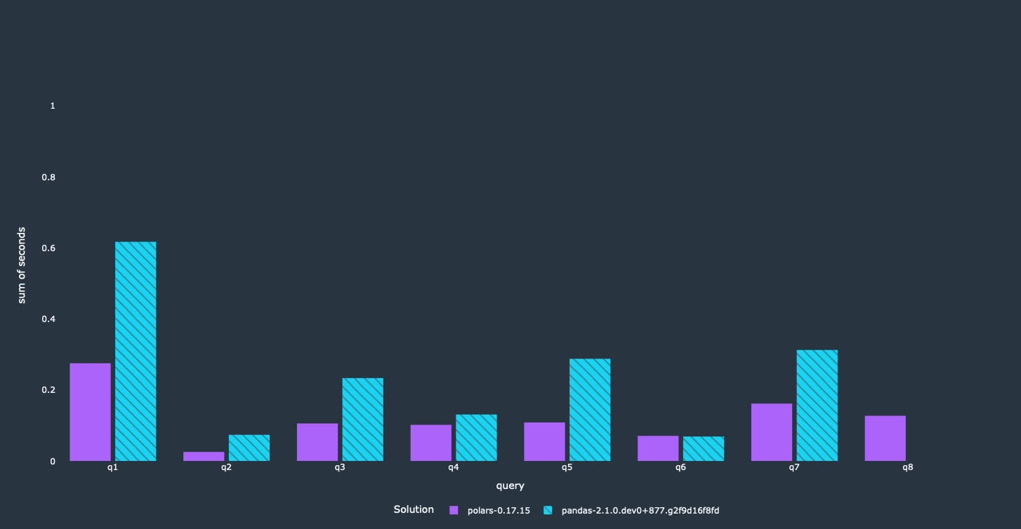
We got a nice performance improvement for most queries. Obviously, this depends on what filter was used in the query itself. Similar to the first optimization, this will reduce the memory footprint significantly, since rows violating the filter won't be loaded into memory at all.

There is one relatively straightforward optimization left without rewriting the queries completely.

Improving merge performance

The following trick requires knowledge about your data and can’t be applied in a general way. This is more of a general idea that isn’t really compliant with tpch rules, but nice to see nevertheless.

This technique is a bit tricky. I stumbled upon this a couple of years ago when I had a performance issue at my previous job. In these scenarios, merge is basically used as a filter that restricts one of both DataFrames quite heavily. This is relatively slow when using merge, because pandas isn't aware that you want to use the merge operation as a filter. We can apply a filter with isin before performing the actual merge to speed up our queries.

import pandas as pd

left = pd.DataFrame({"left_a": [1, 2, 3], "left_b": [4, 5, 6]})
right = pd.DataFrame({"right_a": [1], "right_c": [4]})

left = left[left["left_a"].isin(right["right_a"])]  # restrict the df beforehand
result = left.merge(right, left_on="left_a", right_on="right_a")

This wasn't necessary for all queries, since only a couple of them were using merge in this way. The queries where we applied the technique got another nice performance boost!

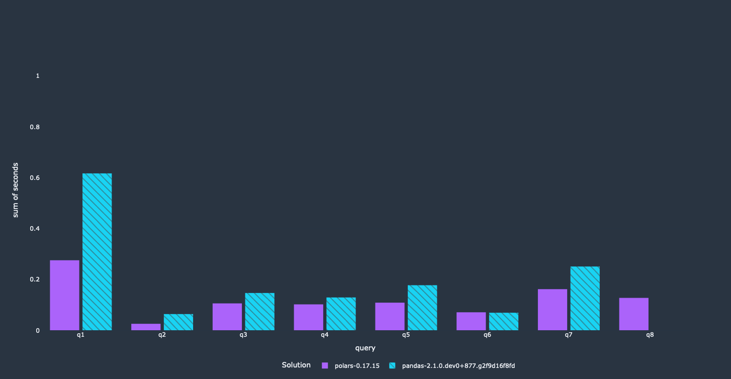
We achieved our main objective here. Most of these queries run a lot faster now than they did before, and use less memory as well. The first query did not get that big of a speedup. It calculates a lot of results on a groupby aggregation, which is done sequentially. We are looking into it right now how we can improve performance here.

Summary

All in all these optimizations took me around 1.5-2 hours. Your mileage might vary, but I don't think that it will take you much longer, since most of the optimizations are very straightforward. A relatively small time investment where most of the time was spent on reorganizing the initial queries. You can find the PR that modifies the benchmarks here. Polars has a query optimization layer, so it does some of these things automatically, but this is not a guarantee that you'll end up with efficient code.

We saw that writing more efficient pandas code isn't that hard and can give you a huge performance improvement. Looking at these queries helped us as well, since we were able to identify a couple of performance bottleneck where we are working on a solution. We were even able to make one of the queries run faster than the Polars version!

These performance improvements mostly translate to the scale_10 version of the benchmarks.

Thanks for reading. Please reach out with any comments or feedback. I wrote a more general post about improving performance in pandas with PyArrow as well.